This post is a gentle overview of our paper. I will present some other interesting results we didn’t include in the paper that might interest the broader audience and the industry.

Introduction

Dynamic malware analysis is the go-to tool for clustering malware into families[1][2][3][4] or detecting malware in cases where static analysis would fail[5][6], such as polymorphic malware. Prior work have proposed techniques to detect malware based off the execution traces[7][8][9][10][11]. However, even with these impressive detection rates, malware outbreaks still happen and pack a serious punch. So there must be some discrepancy between what analyst see in the labs and how malware behave in the wild. In our paper we studied the behavior of malware in the wild, for a dataset collected across 5.4M machines across the globe. In this blog post I will showcase some more results including some case studies. In our work, we answer the following questions:

How much variability is there in malware behavior in the wild across machines and time?
What parts of its behavior varies more?
How does this variability affect existing malware clustering and detection methods?
Can we still find invariants in a malware’s behavior? What parts of the behavior profile are more likely to yield invariants?

For the sake of brevity, in this report I will briefly report our results on questions 1, 3 and 4, while providing some motivating case studies.

Dataset

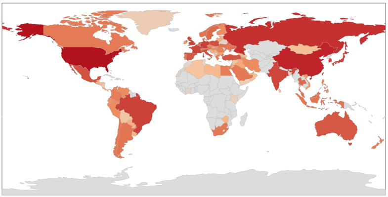
Figure : Figure 1: Number of execution for various countries

We are able to answer all the aforementioned questions through a dataset of program executions, we collected from 5.4M machines across 113 countries. In Figure 1, we show a distribution of the program executions in our dataset. Evidently, the majority comes from USA, China, Russia and the European countries.

OS version	% execs
Win 7 build 7601	56%
Win 10	35%
Win 8.1	3.1%
Win Server	2.6%
Win XP	2%
Other	1.3%

As we see from the table above the most popular windows OS version in 2018 was Win 7 build 7601. This may no longer be the case in 2021 and the threat landscape may not be the same, but the malware behavior must be more evasive. Therefore the behavior variability in the wild should only be higher.

Variability

We measure the variability in terms of missing and additional actions in malware, PUP and benign execution traces across machines and time. In this blog post I will only focus on cross-machine variability.
For more details on the exact definition of variability and other results I would encourage you to check section 2 in the paper.

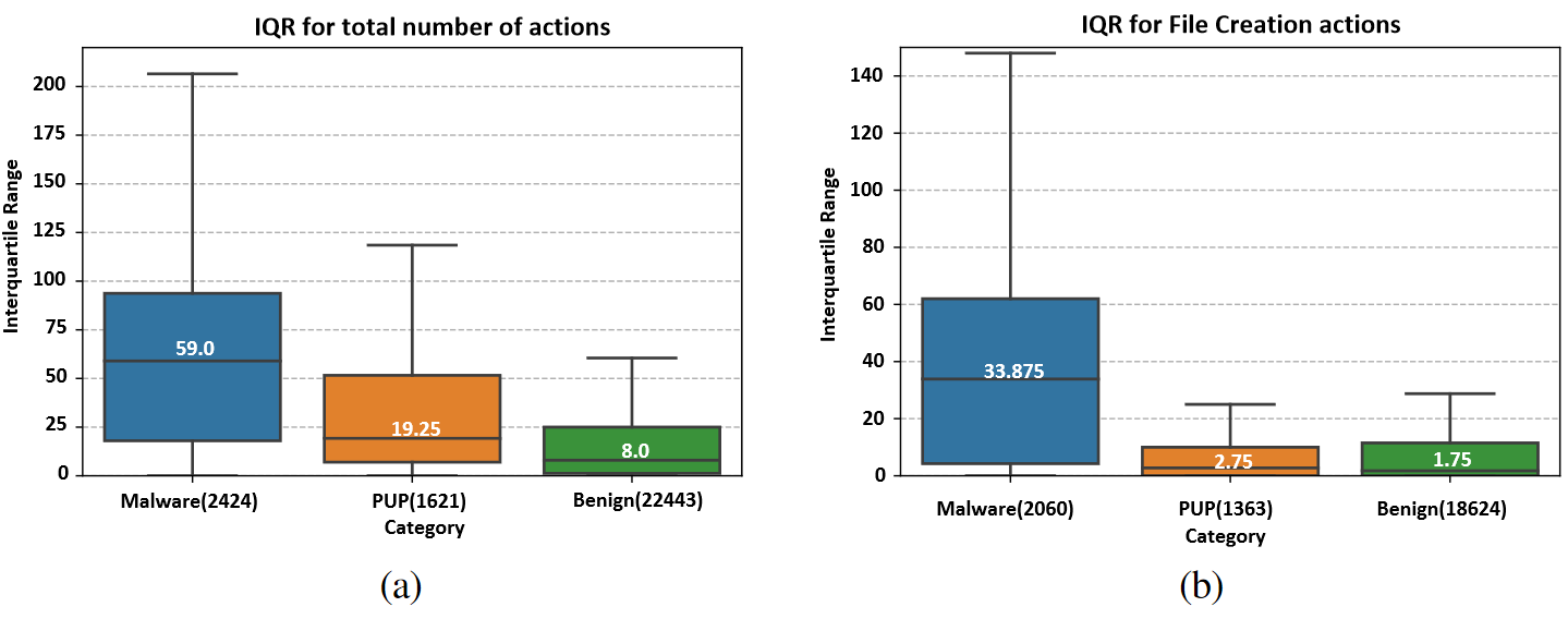
Figure : Figure 2: Number of missing/additional actions across machines in malware, PUP and benign samples.

In the boxplots in Figure 2, we plot the number of missing/addional actions across machines for all malware, PUP and benign samples. As you can see, at least 50% of the malware samples in our dataset have around 59 missing/additional events in the trace where 33 are file creations (Figure 2b).

To better zoom in on this variability we built a Splunk dashboard with information about difference between 2 traces. Below I will present some of the variability we found in the wild and the cause of it.

Case study: The Ramnit worm (VT link)

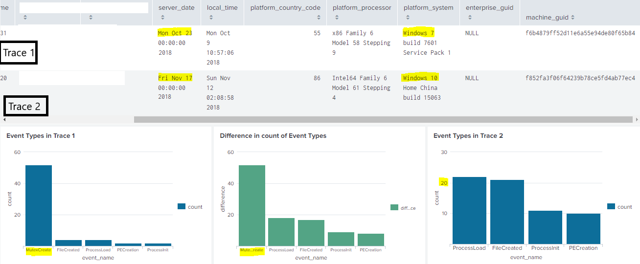
Figure : Figure 3: SPLUNK dashboard showing the comparison of 2 executions of Ramnit on Windows 7 (left) and Windows 10 (right).

An interesting case was that of Ramnit worm. The analysts from cert.pl blog have confirmed that if the Ramnit worm is executed with non-admin privilleges it will try to privillege escalation. In the vulnerable version of Windows 7 it will exploit CVE-2013-3660. From exploit-db we found a confirmed working exploit code, which seems to create mutexes. The large amount of Mutex creations may happen because the malware keeps running the exploit until it succeeds.

Going back to Figure 3, the green bar plot in the middle is the absolute difference in the number of actions for each event type. As we can see from the blue graph on the left, trace 1 has around 50 mutex creation actions while the plot on the right doesn’t have any. This result shows what the analysts of cert.pl blog have manually seen.

This environment-sensitive behavior, however happens very often[12] in malware thus it’s to be expected that the behavior variablity in the wild is the largest among the 3 categories (malware, PUP and benign).

Case study: The Darkcomet RAT (VT link)

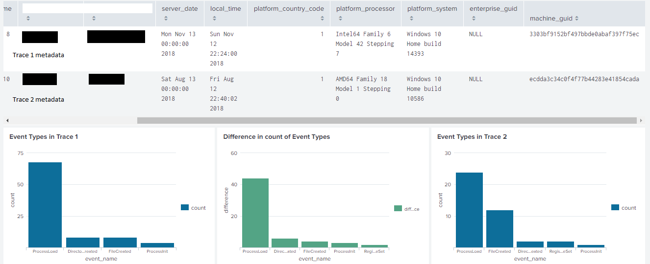
Figure : Figure 4: SPLUNK dashboard showing the comparison of 2 executions of Darkcomet on 2 different times and 2 different machines.

Another case of variability across machines or time is the Darkcomet RAT. In particular case, variabilty is hard to be correctly attributed to a root cause, since the RAT may change its behavior in a specific machine (as instructed by the attacker) or through time if the attacker start an attack campaign (ie. DDoS). Nevertheless, we notice that in trace 2 the malware creates Registry keys while in trace 1 it doesn’t, meanwhile in trace 2 it creates a lot more files. This could be due to new commands issued by the C2.

Invariant

With all this behavior variability can the analyst still detect the malware? We turn our attention to host-based IDS systems (ie. Splunk, Sumo logic, Qradar or other SIEM tools). In this section, we measure the effectiveness of most common

Methodology

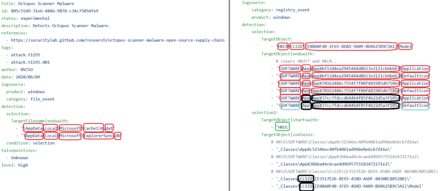
Figure : Figure 5: Tokenization of SIGMA rules' parameters. Octopus Scanner detection rule (left) and OceanLotus Registry activity detection rule (right).

To answer this question, we first scrapped all the rules from Sigma to analyze their composition. In Figure 5, we show 2 SIGMA rules, in which we split the parameters’ values into tokens via windows delimiters. The tokens are shown in red. To highlight the importance of this tokenization we perform it for all the SIGMA rules and we consider a full token to exist if the rule shows 3 tokens with no regular expresssion character in between, this way we eleminate cases where only a part of the token is present, such as the green box. We noticed that around 70% of all the existing open source rules have at least 1 full token in the middle, as shown in black. Considering our approach, this is a lower bound estimate on the true value of full token matching rules.

I’m not highlighting all the tokens with all their resepective colors, but you get the point.

This is important because now we know that if 1 of these tokens is doesn’t match the entire rule will not. So we go back to our dataset and split all the parameters of all our execution actions into windows delimited tokens. Our goal is to analyze the prevalence of these tokens in the wild.

Basically we are not interested in common tokens (ie. exe, windows32, setup, cmd), but in malware-specific tokens (ie. wnry) since the latter will be used in a SIEM signature. Therefore, the first step from our analysis is to remove all tokens that appear in any of the benign samples and all tokens that appear only in 1 machine (randomness). We assume the analyst will use their knowledge or a data-driven method to remove randomness. The leftover from the culling are considered to be malware-specific tokens. We consider the set of all the tokens left as the invariant, since an analyst can create IDS rules that check the presence of at least 1 of the tokens, in the action’s parameter.

The invariant is a bag/set of tokens.

Gotta catch em’ all

The first measurement we conduct is to evaluate the number of minimum number of machines an analyst would need to capture all malware-specific tokens. The question we answer is: How many machines are needed to capture all malware-specific tokens for most common parameters?. We consider common, the parameters most used by the SIGMA rules. Of course, this assumes that the malware author will execute the malware at the perfect time and system to obtain the largest amount of tokens. This estimate is of course a lower bound, but it serves to illustrate the difficulty in obtaining the tokens needed for SIEM signatures.w

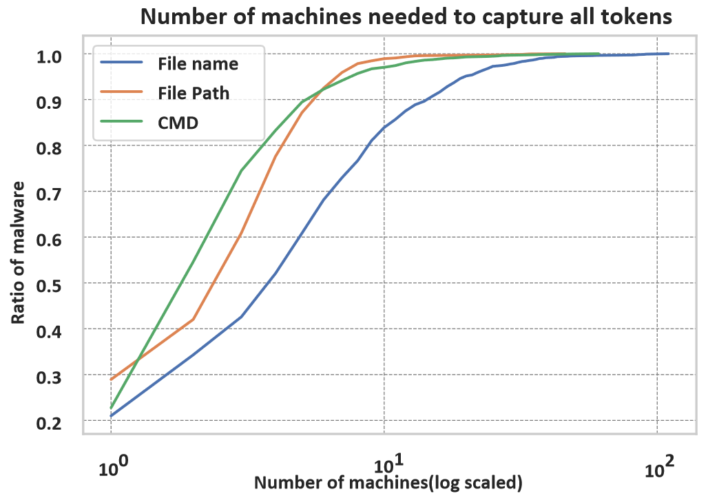
Figure : Figure 6: Number of machines needed to capture all malware-specific tokens.

As we see from Figure 6, for different parameters it requires different amount of machines to get all the values. The hardest to capture seems to be the file name where only around 85% of the malware yield all their malware-specific tokens within 10 machines. In SIGMA, the dropped file’s name makes up for ~12% of the rules.

On the other hand, the command line is used in ~40% of the SIGMA rules and rightfully so. Figure 6 confirms that it takes less machines to get the malware-specific tokens.

How successful in detection are the tokens?

While we show how difficult to catch are some tokes from some of the parameters, we also want to know which tokens are the best to be used in detection. For this we measure the ratio of machines in the wild each malware-specific tokens appears. We name the ratio of machines the token appears in the wild as coverage.

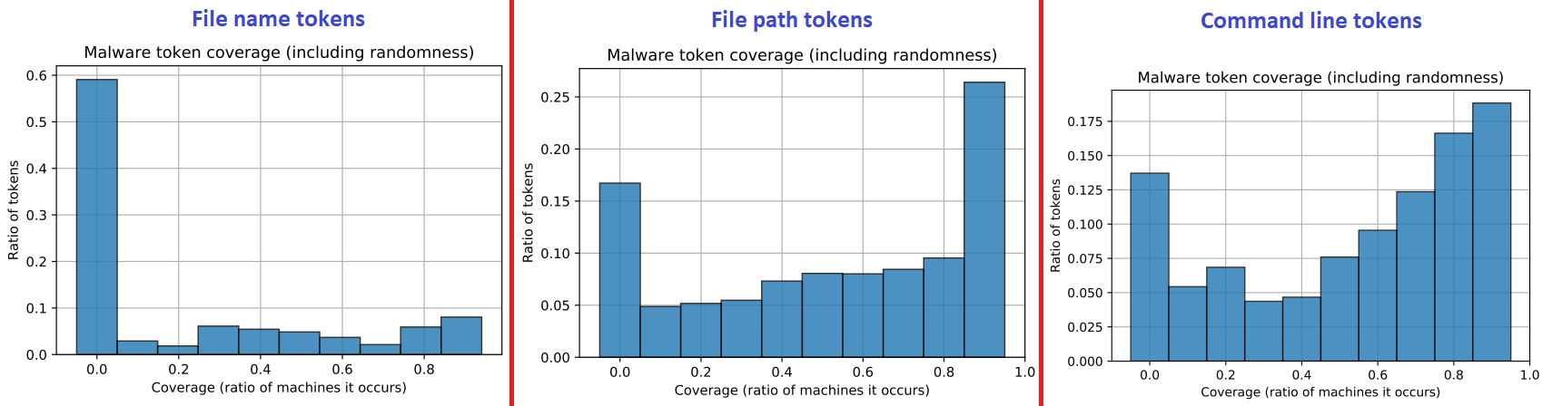
Figure : Figure 7: Coverage of all non-benign tokens (random and malware-specific).

In Figure 7, we measure the coverage of all non-benign tokens an analyst will find in a malware execution trace. The graph can be interpreted as the success rate (coverage) an analyst would get if they picked 1 single random token to make their signature of. Evidently, file path tokens (subdirectories) and command line tokens (CMD parameters) seem to yield better coverage.

But an analyst will not use 1 token and go their merry way. They will pick a all tokens (since by definition they don’t appear in benign samples). In the following sections we will determine how many machines an analyst needs to get the largest coverage. In the paper, we measure how often the analyst needs to reexecute the malware to keep the signatures up-to-date.

Optimal number of machines

In this section we measure the success of detection in the wild, for a set of tokens extracted by N machines. We assume that the malware would behave in the analysts’ sandboxes as if they are running in the wild. The question we answer is: “In how many machines should the analyst execute the malware sample to get the largest coverage of the token set?” We define as coverage, the amount of machines in the wild where 1 of the tokens in the set appears. In a more formal definition, a machine is considered “covered” if the intersection of the “signature” set with the set of tokens in that machine is not empty.

Figure : Figure 8: Total coverage obtained from N machines for 3 most common parameters.

But how can an analyst generate N VMs to resemble N random machines in the wild? - We discuss that an analyst can use a random VM generator like SecGen [13] with the features proposed in Spottless Sandboxes paper [14]. Of course vendors have an idea on the distribution of those features in the wild, so for analysts in such companies generating VMS that resemble the true population of users’ machines in the wild is not a big challenge.

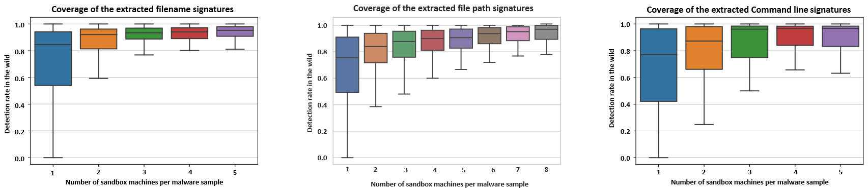
From Figure 8, we notice that an analyst needs to execute the malware sample in 3 machines to get the best coverage using file name tokens. Adding more machines only gives diminishing returns. For more results please refer to our paper.

Effects of behavior variability in malware clustering

As I mentioned earlier, clustering is a very popular method to deal with polymorphic malware samples. Analysts use it to determine if a newly seen executable belongs to a malware family based off the behavior it shows in the sandbox. However, they usually only use 1 execution per malware sample to determine the cluster (ie. malware family) the sample belongs to.

In this section we will analyze how effective clustering is in the wild. The closest clustering paper that uses features similar to ours is that by Bailey et al. [15]. Our goal is not to find the malware families, but to argue the validity of clustering results. The core idea is that executions from the same sample/hash should fall in the same cluster. For that we pick 4 random executions per malware sample and perform the clustering.

number of clusters	% of malware samples
1	67%
2	27%
3	5%
4	1%

Since we pick 4 executions per sample we count the number of clusters those 4 executions fall in. In the table above we show the malware samples for each the 4 executions fall in 1,2,3 and 4 different clusters. We noticed that 33% of the malware samples have executions in 2 different clusters, therefore if we were to interpret each cluster as a malware family it’s not clear which family they belong to. Surprisingly, 1% of the malware have executions in 4 different clusters.

Conclusion

It has been known, for over a decade, that malware samples can change their behavior on different hosts and at different points in time, but no study has yet measured this variability in the real world. In this paper, we report the first analysis of malware, PUP and benign-sample behavior in the wild, using execution traces collected from 5.4M real hosts from around the world. We show that malware exhibits more variability than benign samples. The causes may be different based on the malware type, vulnerabilities in the victims’ machines etc.

We then assess the prevalence of invariant parameter tokens that are commonly used to derive behavior based signatures for malware. Our results suggest that analysts should re-execute the malware samples 3 weeks after first receiving them to update their behavior models.

At last we show that an analyst should be cautious of the malware bahavior variability when clustering them.

Our findings have important implications for malware analysts and sandbox operators, and they emphasize the unique insights that we can gain by monitoring malware behavior at scale, on real hosts.

Any comments of feedback? Please drop a line below 😉